이번 포스팅에서는 TensorBoard의 간단한 사용법에 대해 다양한 tensorflow를 활용한 예시 code와 함께 알아보도록 하겠습니다.
TensorBoard 사용법에 대해 궁금해 하는 사람들 중 TensorFlow를 모르는 사람은 없을 거라 생각하지만 간단히 TensorFlow와 TensorBoard에 대해 살펴보고 Tutorial로 넘어가도록 하겠습니다 :-)
1. TensorFlow? TensorBoard?
TensorFlow
TensorFlow는 Google의 인공지능 연구 조직인 Google Brain 팀이 기계학습(Machine Learning)과 심층 신경망(Deep Neural Network) 연구를 위해 개발한 오픈소스 소프트웨어 라이브러리입니다. TensorFlow는 데이터 플로우 그래프(Data Flow Graph) 방식을 사용하여 모델 내에서 수행되는 방대한 양의 연산과 데이터의 흐름을 표현합니다. 데이터 플로우 그래프는 수학연산을 나타내는 노드(node)와 그 노드들 간의 입/출력 관계를 나타내는 엣지(edge)로 구성되어 있으며, TensorFlow 의 이름에서도 알 수 있듯이 다차원 데이터 배열인 Tensor는 이 엣지들을 통해 노드 간 흐름을 따릅니다.
TensorBoard
TensorFlow는 매우 견고하면서도 유연한 아키텍처를 가지고 있어 별도의 코드 수정 없이 학습 모델을 설계할 수 있고 실행시킬 수 있습니다. 하지만 거대하고 복잡한 뉴럴넷의 코드만을 보고 계산과정이나 데이터의 흐름을 이해하기란 매우 추상적이며 복잡하고 난해할 수 있습니다. 디버깅과 최적화도 매우 어려운 작업이 될 수 있습니다. 이에 TensorFlow는 TensorBoard 라는 시각화 툴을 통해 사용자들이 그래프 내에서 Tensor의 흐름을 쉽게 이해하고, 각 변수들의 양적 변화를 한 눈에 알 수 있도록 돕는 여러 기능을 제공합니다.
2. TensorBoard
Tensor Operation
TensorBoard를 본격적으로 시작하기에 앞서 간단한 TensorFlow 코드를 살펴보겠습니다.
import tensorflow as tf

const1 = tf.constant(3.0, name='const1')
const2 = tf.constant(4.0, name='const2')
print(const1, const2)

add = tf.add(const1, const2)
print(add)

sess = tf.Session()
sess.run(add)
위의 코드를 실행시켜 보면 터미널창에는 아래와 같은 화면이 출력될 것입니다.
Tensor("const1:0", shape=(), dtype=float32) Tensor("const2:0", shape=(), dtype=float32)
Tensor("Add:0", shape=(), dtype=float32)
이처럼 TensorFlow는 Session이 만들어져서 run함수가 호출되기 전까지는 각각의 Tensor 만 생성이 될 뿐 어떠한 연산도 실제로 실행되지 않습니다. 연산에 필요한 모든 Tensor들이 준비된 후 Session이 만들어지고 난 후, 실제 연산은 sess.run(add) 이 한 줄에서 실행됩니다. 위 코드의 마지막줄에 print(sess.run(add))를 추가하여 다시 실행하면 const1과 const2가 add라는 함수로 입력되어 연산된 결과를 확인 할 수 있습니다.
Data Flow Graph
Summary
const1과 const2가 add라는 함수로 입력되어 연산되는 Data Flow Graph 를 TensorBoard를 통해 확인해보겠습니다. 코드는 아래와 같습니다.
import tensorflow as tf
import os

tb_dir = os.path.join(os.getcwd(), "tb_tutorial")
cur_dir = os.path.join(tb_dir, "ex")

const1 = tf.constant(3.0, name='const1')
tf.summary.scalar('const1', const1)

const2 = tf.constant(4.0, name='const2')
tf.summary.scalar('const2', const2)

add = tf.add(const1, const2)
tf.summary.histogram('add', add)

merged = tf.summary.merge_all()

sess = tf.Session()
sess.run([add, merged])

writer = tf.summary.FileWriter(cur_dir, graph=sess.graph)
writer.close()
TensorBoard는 summary operation을 이용하여 저장한 데이터들을 merge한 후 그래프를 시각화합니다. 따라서 우리는 summary operation이 로그 데이터를 저장할 디렉터리를 먼저 생성한 후 튜토리얼을 진행하겠습니다. (line 4~5) 앞으로 진행될 튜토리얼의 모든 로그 데이터들은 tb_tutorial 디렉터리에 각 주제에 맞게 하위 디렉터리를 생성 후 그 곳에 저장하도록 하겠습니다.
TensorBoard는 해당 디렉터리에 로그를 누적하여 저장하며 가장 최근에 저장된 로그를 참고하여 그래프를 그립니다.
line 8, 11, 14를 보면 알 수 있듯이 tf.summary를 이용하여 각 연산자들에 대한 요약 데이터를 저장하고있습니다. 각 summary operation들의 자세한 설명은 여기를 참고하시기 바랍니다. TensorBoard에서도 마찬가지로 각각의 요약 데이터들은 그래프 내에서는 지엽적인 존재입니다. 요약 데이터들을 연결하기 위해서는 merge_all() 함수를 이용하여 모든 요약 데이터들을 하나로 합쳐야 합니다.(line 16) 그러면 모든 요약 데이터를 가지고 있는 summary 프로토버퍼 오브젝트를 생성할 수 있습니다. 우리는 요약 데이터를 디스크에 저장하기 위해 FileWriter에 프로토버퍼 오브젝트를 넘겨줘야합니다. cur_dir로 이벤트 파일이 저장될 디렉터리를 지정해주었고, graph parameter를 설정하여 TensorBoard를 통해 Data Flow Graph를 확인할 예정입니다.(line 21)
위 코드를 실행하면 터미널창에는 아무것도 나타나지 않고, tb_tutorial/ex/ 디렉터리가 생성 된 것을 확인할 수 있을 것입니다. 이제, TensorBoard에서 그래프를 확인하기 위해서 터미널창에 tensorboard --logdir='FileWriter에서_지정한_경로'를 입력해주면 됩니다. 위의 예시코드를 실행한 후 TensorBoard를 확인하는 경우라면 tensorboard --logdir=tb_tutorial/ex/라고 명령어를 입력하시면 됩니다.
logdir 후의 경로가 이벤트 파일이 있는 디렉터리까지 가지 않아도 (이벤트 파일이 있는 디렉터리의 상위 디렉터리여도, 즉 예시의 경우 tb_tutorial까지여도) TensorBoard에서 알아서 구조를 매핑하여 시각화해줍니다.
아무런 에러없이 터미널창에
Strarting TensorBoard at http://localhost:6006과 같은 화면이 출력 됐으면 거의 다 왔습니다. 웹 브라우저를 켜고 주소창에 http://localhost:6006을 입력하신 후 조금 기다리시면 아래와 같은 그래프가 나올 것입니다.
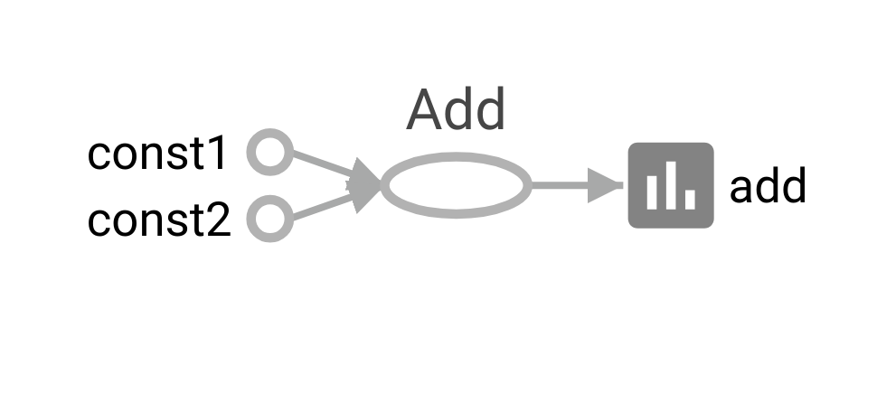
각각의 노드들을 클릭하면 해당 노드에 대한 간단한 description이 오른쪽 상단에 나옵니다. 그래프를 살펴보면 const1과 const2라는 Constant가 Add 연산을 하는 노드의 input으로 들어가 add라는 summary histogram으로 출력되는 Flow 를 볼 수 있습니다.
tensorboard는 logdir 뒤 디렉터리명을 잘못 입력해도 별도의 에러 메시지가 뜨지 않습니다. 현재까지는 path 에러 발생의 유무를 http://localhost:6006 에 접속하여 결과가 표시되는지 확인하는 것 이외에는 별도의 방법이 없습니다 :-(
Simple Operation
또 다른 예시코드를 보겠습니다.
import tensorflow as tf
import os
tb_dir = os.path.join(os.getcwd(), "tb_tutorial")
cur_dir = os.path.join(tb_dir, "power")
a = tf.placeholder(tf.float32)
b = tf.placeholder(tf.float32)
c = tf.placeholder(tf.float32)
multiple = tf.multiply(a, b)
tf.summary.histogram('multiple', multiple)
power = tf.pow(multiple, c)
tf.summary.histogram('power', power)
merged = tf.summary.merge_all()
sess = tf.Session()
print(sess.run([power], feed_dict={a:[1, 2, 3], b:[2, 4, 6], c:2}))
writer = tf.summary.FileWriter(cur_dir, graph=sess.graph)
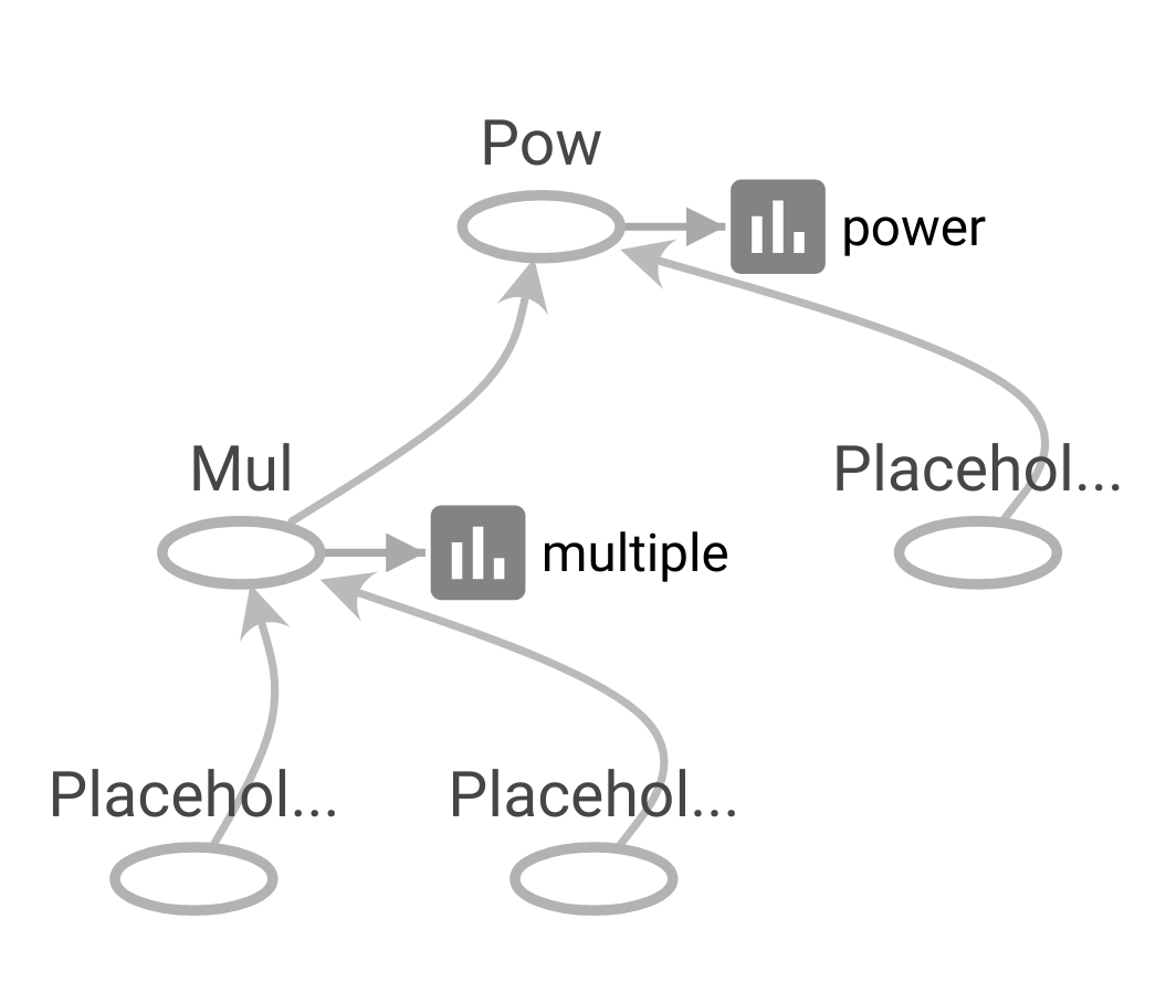
writer.close()위와 마찬가지로 요약 데이터 로그가 저장될 디렉터리를 지정해 준 뒤(line 4~5), a, b, c라는 placeholder를 생성하고 곱셈 연산 노드와 지수연산 노드를 생성해 줍니다. 노드들을 생성할 때마다 summary로 연산자의 요약 데이터도 생성해 준 뒤(line 7~15), 연산의 마지막 단계에서 merge_all 함수를 호출해줍니다(line 17). Session을 생성 한 뒤 run 함수를 이용하여 연산을 실행합니다. 이때, a, b, c에 들어갈 값을 feed_dict 로 지정해줍니다(line 18~19). FileWriter를 이용해 코드 도입부분에서 지정해준 디렉터리에 이벤트 파일을 저장해줍니다(line20~21). 코드를 실행하였으면 이제 터미널창으로 돌아가서 tensorboard --logdir='FileWriter에서_지정한_경로' 를 입력한 후 웹 브라우저 주소창에 http://localhost:6006 입력하여 tensorboard에 나오는 그래프를 확인합니다.
Complex Operation - Linear Regression
이번에는 연산 노드가 앞선 예제들보다 조금 더 많은 선형회귀 예제 코드를 TensorBoard로 그려보겠습니다.
import tensorflow as tf
import numpy as np
import os

tb_dir = os.path.join(os.getcwd(), "tb_tutorial")
cur_dir = os.path.join(tb_dir, "fahrenheit_converter")

x_data = [12.0, 28.0, 36.5, 42.0, 29.8]
y_data = [53.6, 82.4, 97.7, 107.6, 85.64]

def norm(data):
    #input으로 들어오는 섭씨온도를 정규화해주는 함수
    #x값을 정규화해주지 않으면 학습과정 중 w값과 b값이 양의 무한대, 음의 무한대로 튀는 현상을 발견할 수 있습니다.
    data = np.array(data)
    x_norm = np.zeros([len(data)])
    for i in range(len(data)):
        x_norm[i] = data[i] / 100
    return np.reshape(x_norm, [-1, 1])


x_data = norm(x_data)
y_data = np.reshape(y_data, [-1, 1])


x = tf.placeholder(tf.float32, shape=[None,1])
y = tf.placeholder(tf.float32, shape=[None,1])

W = tf.Variable(tf.random_normal([1,1]), name='weight')
b = tf.Variable(tf.random_normal([1]), name='bias')

hypothesis = tf.add(tf.matmul(x, W), b)

cost = tf.reduce_mean(tf.square(y - hypothesis))

optimizer = tf.train.GradientDescentOptimizer(learning_rate=0.01)
train = optimizer.minimize(cost)

merged = tf.summary.merge_all()

sess = tf.Session()
sess.run(tf.global_variables_initializer())

for step in range(30001):
    _cost, _W, _b, _ = sess.run([cost, W, b, train],
                                feed_dict={x:x_data, y:y_data})
    if step % 1000 == 0:
        print("Step:", step, "\tCost:", _cost,
              "\tW:", _W[0], "\tb:", _b)

writer = tf.summary.FileWriter(cur_dir, graph=sess.graph)
writer.close()

print("X: 20, Y:", sess.run(hypothesis[0], feed_dict={x:norm([20])}))
print("X: 30, Y:", sess.run(hypothesis[0], feed_dict={x:norm([30])}))
print("X: 40, Y:", sess.run(hypothesis[0], feed_dict={x:norm([40])}))
print("X: 50, Y:", sess.run(hypothesis[0], feed_dict={x:norm([50])}))
print("X: 60, Y:", sess.run(hypothesis[0], feed_dict={x:norm([60])}))
실행결과
...
Step: 27000 	Cost: 0.00965826 	W: [ 179.03100586] 	b: [ 32.29016876]
Step: 28000 	Cost: 0.00663723 	W: [ 179.19673157] 	b: [ 32.24048233]
Step: 29000 	Cost: 0.00455425 	W: [ 179.33456421] 	b: [ 32.1991806]
Step: 30000 	Cost: 0.00312983 	W: [ 179.44841003] 	b: [ 32.16521835]
X: 20, Y: [ 68.05490112]
X: 30, Y: [ 85.9997406]
X: 40, Y: [ 103.94458008]
X: 50, Y: [ 121.88941956]
X: 60, Y: [ 139.83427429]
위 코드는 섭씨온도를 입력하면 화씨온도를 예측하는 선형회귀식
의 와 를 구하는 코드입니다. Linear Regression을 TensorFlow로 구현하는 코드에 대한 설명은 본 튜토리얼에서는 생략하도록 하겠습니다.
섭씨온도를 화씨온도로 변환하는 공식은 아래와 같습니다.
위 코드를 실행한 후 TensorBoard로 확인하면 아래와 같은 그래프가 생성된 것을 확인할 수 있습니다.
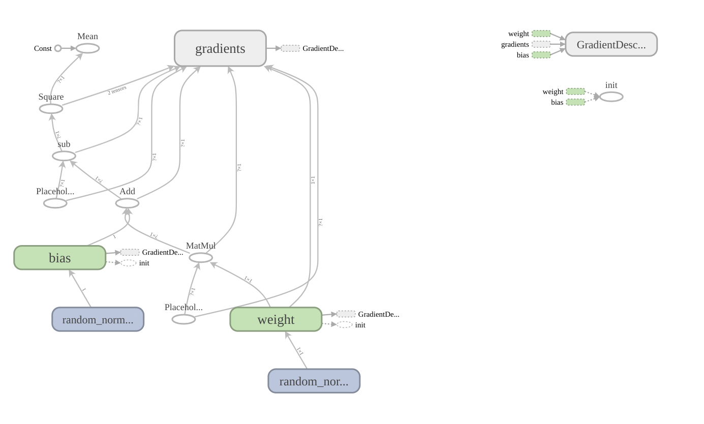
앞서 봤던 단순한 add 연산이나 power연산의 그래프보다 노드가 훨씬 많아졌고, gradients, weight, bias 와 같은 namespace가 생성된 것을 확인할 수 있습니다. 각각의 namespace를 더블 클릭하면 내부의 또다른 복잡한 노드들 간의 flow를 볼 수 있습니다. gradients 같은 경우에는 namespace 안에 또 여러개의 namespace가 있습니다. 엣지에도 각 노드로 입/출력 되는 tensor의 shape에 대한 정보가 쓰여있습니다.
Histogram
위의 코드를 실행했을 때, step이 증가할때마다 cost , W , b 의 값이 업데이트 되는 것을 확인할 수 있었습니다. TensorBoard에서는 histogram 으로 변수에 할당된 값의 변화를 저장하고 그 값을 한번에 모아서 한 그래프에 보여주는 기능을 제공합니다. 위의 코드에 단 몇줄만 추가하면 변화량을 시각화하여 볼 수 있습니다.
아래 예시부터는 코드의 변화가 있을 때마다 이벤트 파일을 저장하는 디렉터리를 다르게 지정하여 전후 코드 간 비교 가능하게 하였습니다. 디렉터리 지정은 TensorBoard 사용자 임의대로 할 수 있습니다. 또한
...으로 생략한 부분은 동일 내용의 코드입니다. 본 tutorial에서 사용한 모든 코드는 이 곳에서 확인가능 합니다.
...
W = tf.Variable(tf.random_normal([1,1]), name='weight')
tf.summary.histogram('weight', W)

b = tf.Variable(tf.random_normal([1]), name='bias')
tf.summary.histogram('bias', b)

hypothesis = tf.add(tf.matmul(x, W), b)

cost = tf.reduce_mean(tf.square(y - hypothesis))
tf.summary.histogram('cost', cost)
...
W , b 와 cost 에 해당하는 histogram 요약 데이터를 생성하였습니다. 이제 학습을 진행하면서 값이 변화하고 그 변화를 histogram 그래프에 나타내야 하기 때문에 step마다 요약 데이터를 기록해야 합니다. 아래에서 코드를 조금 더 수정하도록 하겠습니다.
...
sess = tf.Session()
sess.run(tf.global_variables_initializer())

writer = tf.summary.FileWriter(cur_dir, graph=sess.graph)
merged = tf.summary.merge_all()

for step in range(30001):
    _merged, _cost, _W, _b, _ = sess.run([merged, cost, W, b, train],
                                         feed_dict={x:x_data, y:y_data})
    writer.add_summary(_merged, global_step=step)
    if step % 1000 == 0:
        print("Step:", step, "\tCost:", _cost,
              "\tW:", _W[0], "\tb:", _b)

writer.close()
...
업데이트 되는 요약 데이터를 계속 저장해줘야 하기 때문에 FileWriter를 학습시작 전에 실행시켜주었고, 학습의 step이 증가할 때마다 요약 데이터를 add_summary를 이용하여 기록해주고 있습니다. 이제 다시 터미널창으로 가서 tensorboard를 활성화하는 명령어를 입력해주고 tensorboard를 확인해봅니다.
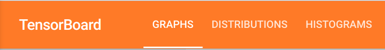
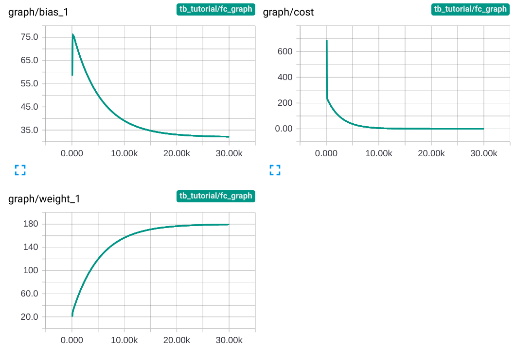
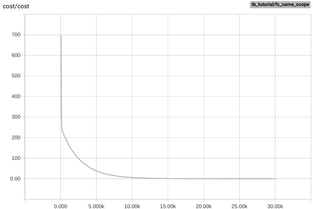
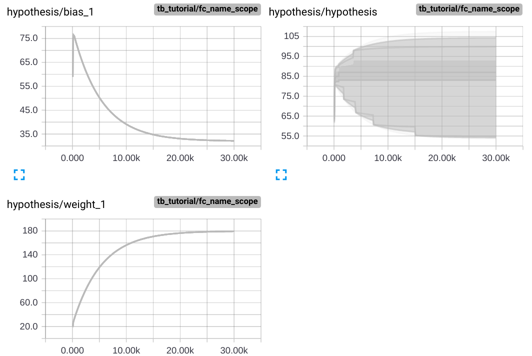
Main Graph에는 변화가 없지만 상단의 navigation bar에 Distribution 과 Histogram tab이 생성된 것을 확인할 수 있습니다. Distribution tab에서는 아래와 같은 그래프들을 확인할 수 있습니다.
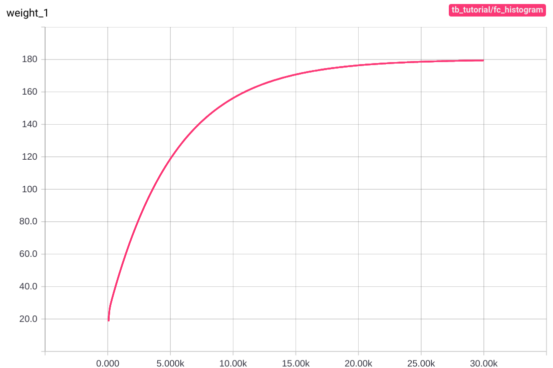
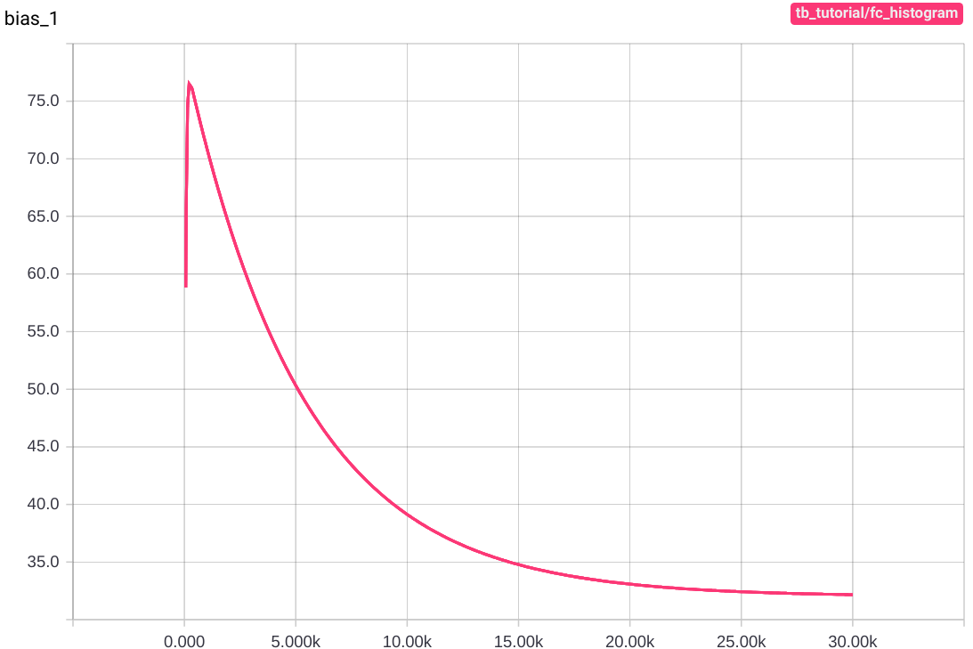
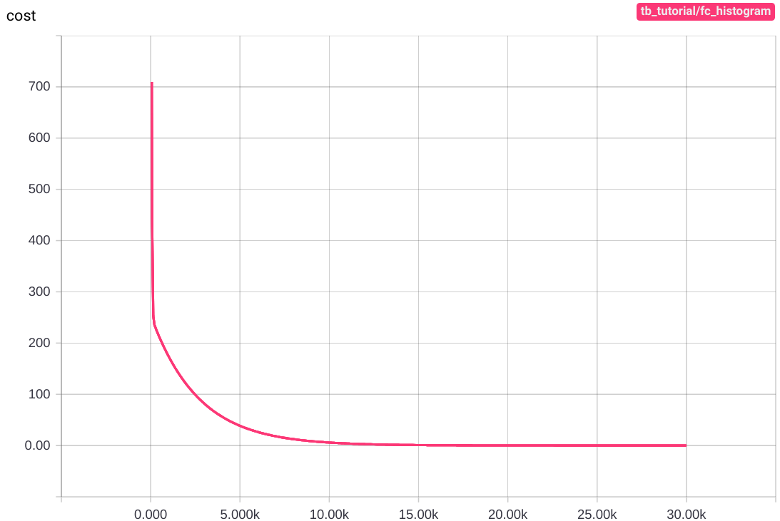
그래프의 세로축은 각각 weight, bias, cost의 step마다의 값이고 가로축은 step 수 입니다. 학습을 거듭할 수록 cost는 0에 가까워지고, weight와 bias는 각각 180과 32에 가까워집니다.
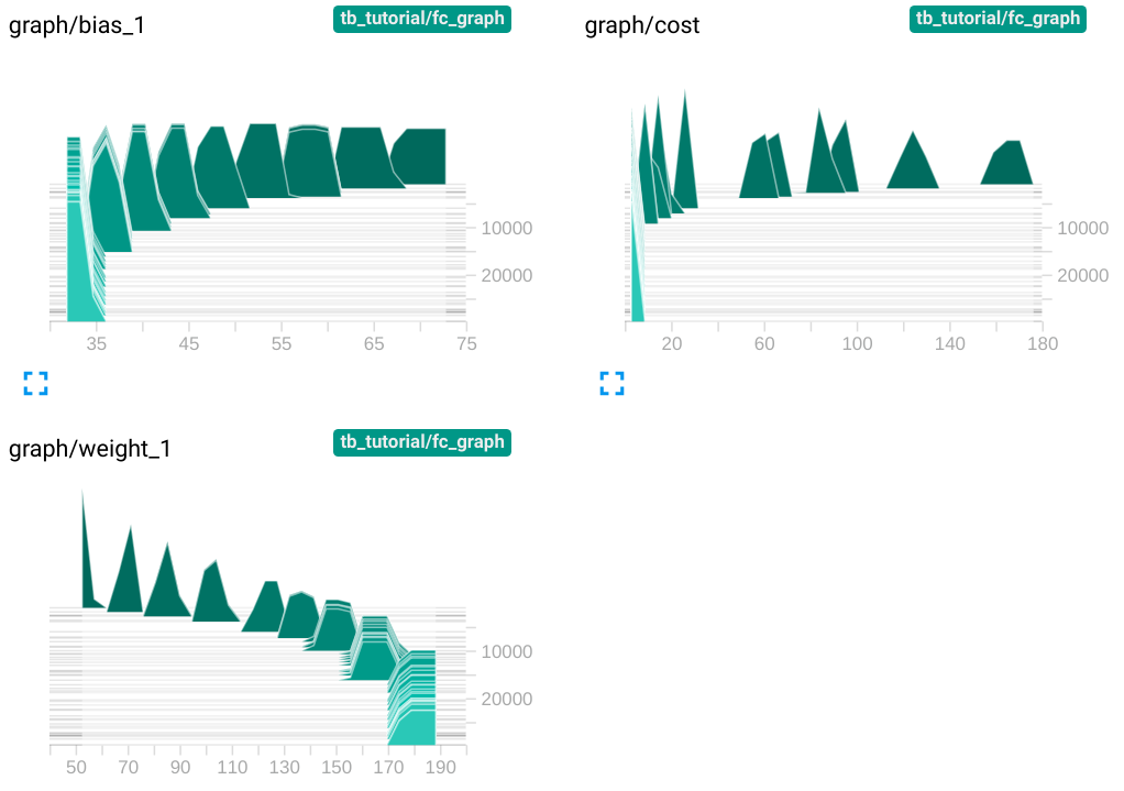
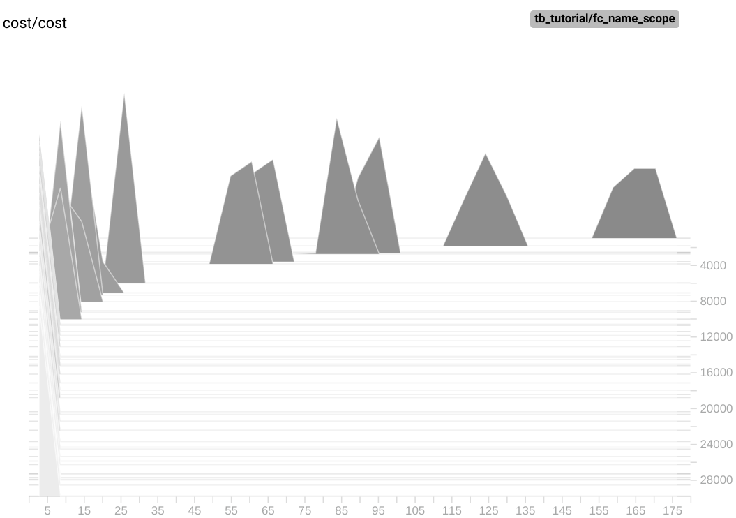
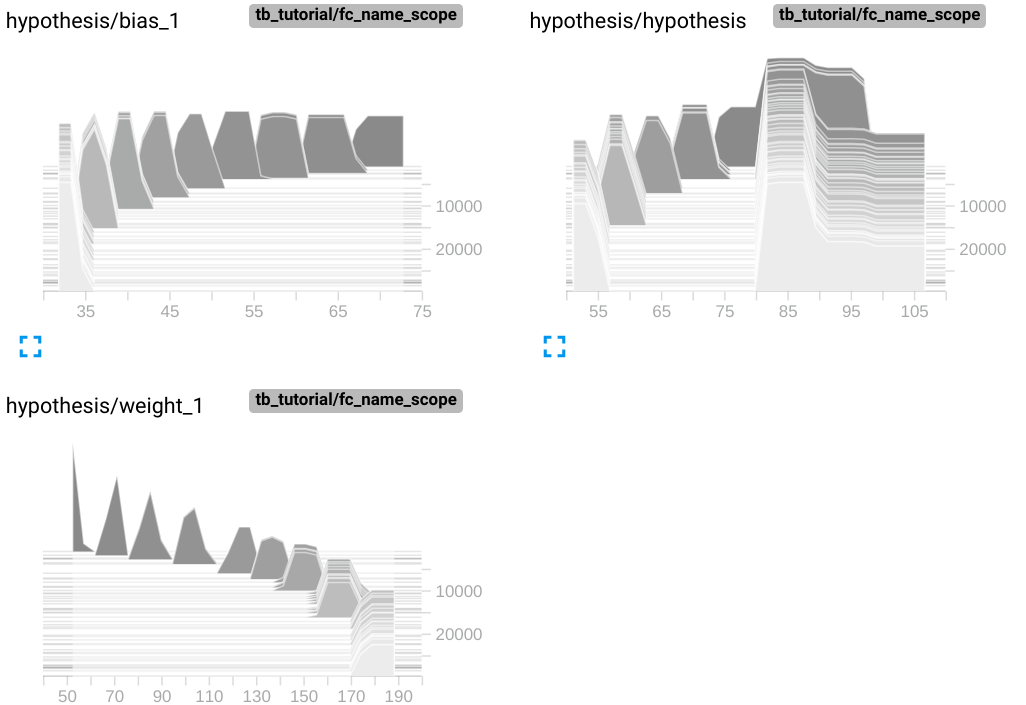
Histogram tab에서는 아래와 같은 그래프들을 확인할 수 있습니다.
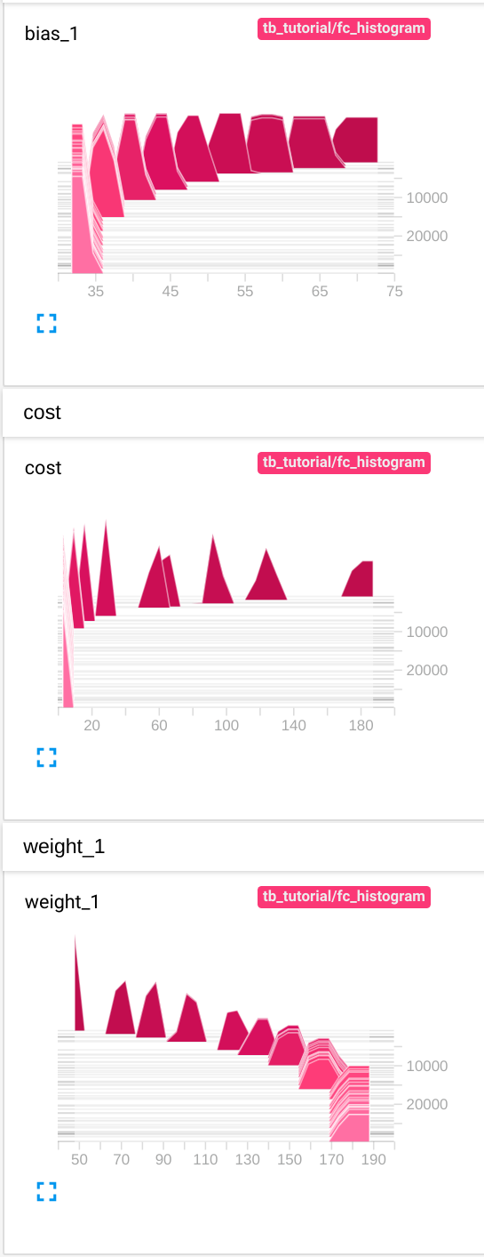
Histogram 그래프는 가로축이 bias, cost, weight 각각의 step마다의 값을, 세로축이 학습횟수를 의미합니다. 그래프가 여러겹 중첩된 것을 확인할 수 있지만 값들의 분포가 무엇을 의미하는지는 정확히 알 수 없습니다.
Name Scope
우리는 앞에서 gradients라는 namespace가 자동으로 생성된 것을 확인할 수 있었습니다. TensorBoard에서는 사용자도 namespace를 생성할 수 있게 하였는데, 그것이 바로 name_scope 입니다. name_scope을 이용하여 원하는 노드들을 한 데 묶어 하나의 namespace로 생성할 수 있습니다. 위의 코드에 단 한줄만 추가하면 우리는 fahrenheit_converter의 복잡한 Data Flow Graph를 하나의 namespace로 묶을 수 있습니다.
...
with tf.name_scope('graph') as scope:
W = tf.Variable(tf.random_normal([1,1]), name='weight')
tf.summary.histogram('weight', W)
b = tf.Variable(tf.random_normal([1]), name='bias')
tf.summary.histogram('bias', b)
hypothesis = tf.add(tf.matmul(x, W), b)
cost = tf.reduce_mean(tf.square(y - hypothesis))
tf.summary.histogram('cost', cost)
optimizer = tf.train.GradientDescentOptimizer(learning_rate=0.01)
train = optimizer.minimize(cost)
sess = tf.Session()
sess.run(tf.global_variables_initializer())
writer = tf.summary.FileWriter(cur_dir, graph=sess.graph)
merged = tf.summary.merge_all()
for step in range(30001):
_merged, _cost, _W, _b, _ = sess.run([merged, cost, W, b, train],
feed_dict={x:x_data, y:y_data})
writer.add_summary(_merged, global_step=step)
if step % 1000 == 0:
print("Step:", step, "\tCost:", _cost, "\tW:", _W[0], "\tb:", _b)
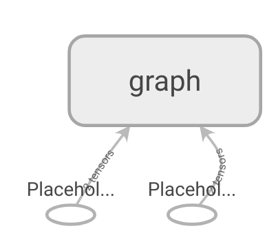
writer.close()with tf.name_scope('graph') as scope: 라는 한줄을 namespace로 묶고자 하는 노드 전에 선언해주기만 하면 끝입니다. name_scope의 인자로 들어가는 'graph'는 TensorBoard에서 보여질 namespace의 이름입니다. name_scope 으로 묶인 노드들은 distribution graph와 histogram graph에서도 묶여서 그려집니다.
name_scope은 원하는 만큼 사용할 수 있습니다. 위의 코드에서 Hypothesis , Cost , Train 으로 나눠서 name_scope을 지정해준 뒤 TensorBoard로 확인해보겠습니다.
...
with tf.name_scope('hypothesis') as scope:
    W = tf.Variable(tf.random_normal([1, 1]), name='weight')
    tf.summary.histogram('weight', W)

    b = tf.Variable(tf.random_normal([1]), name='bias')
    tf.summary.histogram('bias', b)

    hypothesis = tf.add(tf.matmul(x, W), b)
    tf.summary.histogram('hypothesis', hypothesis)

with tf.name_scope('cost') as scope:
    cost = tf.reduce_mean(tf.square(y - hypothesis))
    tf.summary.histogram('cost', cost)

with tf.name_scope('train') as scope:
    optimizer = tf.train.GradientDescentOptimizer(learning_rate=0.01)
    train = optimizer.minimize(cost)

    sess = tf.Session()
    sess.run(tf.global_variables_initializer())

    writer = tf.summary.FileWriter(cur_dir, graph=sess.graph)
    merged = tf.summary.merge_all()

    for step in range(30001):
        _merged, _cost, _W, _b, _ = sess.run([merged, cost, W, b, train],
                                              feed_dict={x: x_data, y: y_data})
        writer.add_summary(_merged, global_step=step)
        if step % 1000 == 0:
            print("Step:", step, "\tCost:", _cost, "\tW:", _W[0], "\tb:", _b)

    writer.close()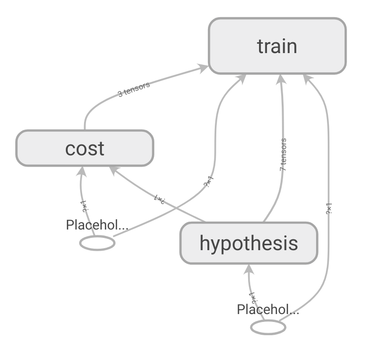
MNIST CNN with TensorBoard!!
여러분들은 TensorBoard의 여러 기능들 중 기계학습과 심층 신경망 학습에 최소한으로 필요한 기능들에 대해서 다 배웠습니다! 여러 기능들이 더 있지만 이 기본적인 operation 들로 CNN MNIST Classifier 의 Data Flow Graph를 볼 수 있습니다. 예시코드는 김성훈 교수님의 MNIST CNN code를 참고하였습니다.
import tensorflow as tf
from tensorflow.examples.tutorials.mnist import input_data
import os

tb_dir = os.path.join(os.getcwd(), "tb_tutorial")
cur_dir = os.path.join(tb_dir, "mnist_cnn")

tf.set_random_seed(777)

mnist = input_data.read_data_sets("MNIST_data/", one_hot=True)

learning_rate = 0.001
training_epochs = 15
batch_size = 100

x = tf.placeholder(tf.float32, [None, 784])
x_img = tf.reshape(x, [-1, 28, 28, 1])
y = tf.placeholder(tf.float32, [None, 10])

with tf.name_scope('conv1') as scope:
    W1 = tf.Variable(tf.random_normal([3, 3, 1, 32], stddev=0.01))

    L1 = tf.nn.conv2d(x_img, W1, strides=[1, 1, 1, 1], padding='SAME')
    L1 = tf.nn.relu(L1)
    L1 = tf.nn.max_pool(L1, ksize=[1, 2, 2, 1],
                        strides=[1, 2, 2, 1], padding='SAME')

with tf.name_scope('conv2') as scope:
    W2 = tf.Variable(tf.random_normal([3, 3, 32, 64], stddev=0.01))

    L2 = tf.nn.conv2d(L1, W2, strides=[1, 1, 1, 1], padding='SAME')
    L2 = tf.nn.relu(L2)
    L2 = tf.nn.max_pool(L2, ksize=[1, 2, 2, 1],
                        strides=[1, 2, 2, 1], padding='SAME')
    L2_flat = tf.reshape(L2, [-1, 7*7*64])

with tf.name_scope('fc') as scope:
    W3 = tf.get_variable("W3", shape=[7*7*64, 10],
                         initializer=tf.contrib.layers.xavier_initializer())
    tf.summary.histogram("weight", W3)

    b = tf.Variable(tf.random_normal([10]))
    tf.summary.histogram("bias", b)

    logits = tf.matmul(L2_flat, W3) + b
    tf.summary.histogram('logits', logits)

with tf.name_scope('train') as scope:
    cost = tf.reduce_mean(tf.nn.softmax_cross_entropy_with_logits(logits=logits,labels=y))
    tf.summary.histogram('cost', cost)

    optimizer = tf.train.AdamOptimizer(learning_rate=learning_rate)
    train = optimizer.minimize(cost)

    sess = tf.Session()
    sess.run(tf.global_variables_initializer())

    writer = tf.summary.FileWriter(cur_dir, graph=sess.graph)
    merged = tf.summary.merge_all()

    for epoch in range(training_epochs):
        avg_cost = 0
        total_batch = int(mnist.train.num_examples / batch_size)

        for i in range(total_batch):
            batch_xs, batch_ys = mnist.train.next_batch(batch_size)
            feed_dict = {x:batch_xs, y:batch_ys}
            _merged, _cost, _ = sess.run([merged, cost, train],
                                          feed_dict=feed_dict)
            writer.add_summary(_merged, global_step=epoch*i)
            avg_cost += _cost / total_batch
        print('Epoch:', '%04d' % (epoch + 1), 'cost =', '{:.9f}'.format(avg_cost))
위 코드를 살펴본 후 run하고, TensorBoard를 실행하여 어떤 Graph와 Distribution, Histogram이 그려졌는지 확인해보세요! 지금까지 읽어주시고 같이 실습해주셔서 (안해주셨어도) 감사합니다.
References