이 포스팅에는 kaggle에서 제공하는 raw data 를 전처리하는 과정과 Word2Vec 모델을 이용하여 vectorizing 하는 과정이 포함되어있습니다. 코드 작성은 python3와 pandas. sklearn, gensim 을 이용했습니다.
Exploring data
데이터의 분포를 살펴보며 어떤 모델이 적합할 지 생각합니다.
what’s cooking 의 train data는 다음과 같은 형식으로 주어집니다.
{
"id": 24717,
"cuisine": "indian",
"ingredients": [
    "tumeric",
    "vegetable stock",
    "tomatoes",
    "garam masala",
    "naan",
    "red lentils",
    "red chili peppers",
    "onions",
    "spinach",
    "sweet potatoes"
]
},
pandas 라이브러리를 이용해 DataFrame 으로 만든 뒤 데이터의 끝에서부터 3rows 만 살펴보면 다음과 같습니다
import pandas as pd
import numpy as np
import sklearn
import matplotlib.pyplot as plot
data=pd.read_json("train.json")
df = pd.DataFrame(data)
df.tail(3)
| cuisine | id | ingredients |
|---|---|---|
| irish | 2238 | [‘eggs’, ‘citrus fruit’, ‘raisins’, ‘sourdough starter’, ‘flour’, ‘hot tea’, ‘sugar’, ‘ground nutmeg’, ‘salt’, ‘ground cinnamon’, ‘milk’, ‘butter’] |
| chinese | 41882 | [‘boneless chicken skinless thigh’, ‘minced garlic’, ‘steamed white rice’, ‘baking powder’, ‘corn starch’, ‘dark soy sauce’, ‘kosher salt’, ‘peanuts’, ‘flour’, ‘scallions’, ‘Chinese rice vinegar’, ‘vodka’, ‘fresh ginger’, ‘egg whites’, ‘broccoli’, ‘toasted sesame seeds’, ‘sugar’, ‘store bought low sodium chicken stock’, ‘baking soda’, ‘Shaoxing wine’, ‘oil’] |
| mexican | 2362 | [‘green chile’, ‘jalapeno chilies’, ‘onions’, ‘ground black pepper’, ‘salt’, ‘chopped cilantro fresh’, ‘green bell pepper’, ‘garlic’, ‘white sugar’, ‘roma tomatoes’, ‘celery’, ‘dried oregano’] |
이번에는 각 cuisine의 갯수의 분포를 알아보겠습니다.
pandas 의 pivot_table 함수를 사용해서 각 cuisne에 해당하는 row의 갯수를 확인해보겠습니다
cuisine_count=pd.pivot_table(df, index=["cuisine"], values=["id"], aggfunc='count')
실행결과
| cuisine | count |
|---|---|
| brazilian | 467 |
| british | 804 |
| cajun_creole | 1546 |
| chinese | 2673 |
| filipino | 755 |
| greek | 1175 |
| indian | 3003 |
| irish | 667 |
| italian | 7838 |
| jamaican | 526 |
| japanese | 1423 |
| korean | 830 |
| mexican | 6438 |
| moroccan | 821 |
| russian | 489 |
| southern_us | 4320 |
| spanish | 989 |
| thai | 1539 |
| vietnamese | 825 |
matplotlib 을 이용하여 시각화하여 나타내어보면 아래의 그래프와 같은 결과가 나옵니다.
df['cuisine'].value_counts().plot(kind= 'bar')
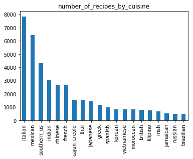
상위 3 종류의 cuisine 이 전체 39774 rows의 약 반 정도를 차지하고 있음을 알 수 있습니다.
Data Preprocessing
- textcase를 일치시켜 줍니다.
- 정규식을 이용하여 특수문자를 모두 제거해줍니다.
- 숫자도 제거해줍니다
- oz 등 재료 단위와 crushed/ground 등 의 단어도 제거해줍니다.
- nltk package 를 이용하여 ingredient들을 모두 단어의 기본형으로 바꿔줍니다 (ex.tomatoes -> tomato)
def clean_recipe(recipe): # 소문자로 변환
    recipe = [ str.lower(i) for i in recipe ]

    def replacing(word): # 알파벳과 띄어쓰기 이외의 문자 모두 제거, crushed, crumbles, diced 등의 단어와 oz, lb와 같은 단위도 모두 제거
        word = re.sub("[^a-z A-Z]","", word)
        word =  re.sub(r'\|crushed|crumbles|ground|minced|powder|chopped|sliced|cut|oz|lb|diced|fried|boneless|skinless|','', word)
        return word

    recipe = [ replacing(i) for i in recipe ]

    # 숫자 제거
    recipe = [ i for i in recipe if not i.isdigit() ]

    # tomatoes -> tomato 와 같이 기본형으로 변환
    for i in recipe:
        buffer = ''
        temp=i.split(' ')
        for k in temp:
            recipe = stemmer.lemmatize(k)
            buffer= buffer +' '+ recipe

        one_recipe.append(buffer)
    return one_recipe
프로세싱 후 df에 cleaned_ingredient라는 새로운 column에 결과를 넣어 확인하면 다음과 같은 결과를 얻을 수 있습니다.
| cuisine | id | flatten_ingredients | cleaned_ingredients |
|---|---|---|---|
| irish | 2238 | eggs,citrus fruit,raisins,sourdough starter,flour,hot tea,sugar,ground nutmeg,salt,ground cinnamon,milk,butter | egg,citrus fruit,raisin,sourdough starter,flour,hot tea,sugar,nutmeg,salt,cinnamon,milk,butter |
| chinese | 41882 | boneless chicken skinless thigh,minced garlic,steamed white rice,baking powder,corn starch,dark soy sauce,kosher salt,peanuts,flour,scallions,Chinese rice vinegar,vodka,fresh ginger,egg whites,broccoli,toasted sesame seeds,sugar,store bought low sodium chicken stock,baking soda,Shaoxing wine,oil | chicken thigh,garlic,steamed white rice,baking,corn starch,dark soy sauce,kosher salt,peanut,flour,scallion,chinese rice vinegar,vodka,fresh ginger,egg white,broccoli,toasted sesame seed,sugar,store bought low sodium chicken stock,baking soda,shaoxing wine,oil |
| mexican | 2362 | green chile,jalapeno chilies,onions,ground black pepper,salt,chopped cilantro fresh,green bell pepper,garlic,white sugar,roma tomatoes,celery,dried oregano | green chile,jalapeno chilies,onion,black pepper,salt,cilantro fresh,green bell pepper,garlic,white sugar,rom tomato,celery,dried oregano |
cleaned_ingredients 로 bag of word 를 생성하는 코드는 다음과 같습니다.
from collections import Counter
bag_of_words = []
for i in range(len(df.id)):
    bag_of_words.append(Counter(df.cleaned_ingredients[i].split(',')))
print(bag_of_words[-1])
실행 결과
[Counter({'black pepper': 1,
          'celery': 1,
          'cilantro fresh': 1,
          'dried oregano': 1,
          'garlic': 1,
          'green bell pepper': 1,
          'green chile': 1,
          'jalapeno chilies': 1,
          'onion': 1,
          'rom tomato': 1,
          'salt': 1,
          'white sugar': 1})]
위와 같은 39774 개의 counter 가 만들어지고 이 bag_of_words 를 이용해 새로운 dataframe을 만들면 모든 ingredient가 column인 39774 * 6439 형태의 dataframe이 생성됩니다.
(전처리 함수(clean_recipe)실행 전 raw data로 bag of word를 만들면 6714개의 column이 존재합니다)
bags = pd.DataFrame(bag_of_words, index =df.id)
bags=bags.fillna(0)
bags.drop([''], axis = 1,  inplace = True)
각 column 별로 sum을 하면 각 ingredient의 출현 횟수를 알 수 있습니다.
sumbags = sum(bag_of_words, Counter())
sumbags.most_common()[:15]  #출현 빈도가 높은 상위 15개 ingredients 출력
실행 결과
[('salt', 18049),
 ('garlic', 10759),
 ('onion', 10182),
 ('olive oil', 7972),
 ('water', 7457),
 ('black pepper', 7412),
 ('sugar', 6434),
 ('garlic clove', 6237),
 ('tomato', 5006),
 ('butter', 4848),
 ('pepper', 4823),
 ('allpurpose flour', 4632),
 ('vegetable oil', 4385),
 ('cumin', 3700),
 ('green onion', 3550)]
전처리를 끝낸 후 각 ingredient별 출현 횟수를 살펴본 결과 소금, 마늘, 양파, 올리브오일 순으로 가장 많이 출현하는 것을 확인할 수 있습니다.
Word2Vec Modeling
from gensim.models import word2vec

# 파라미터 설정
num_features = 300    # wordvector 차원
min_word_count = 3    # 최소 3번 출현한 단어 반영
num_workers = 4       # 병렬처리
context = 10          # window 사이즈
downsampling = 1e-3   # 빈번히 등장하는 단어 downsampling


# Initialize and train the model
model = word2vec.Word2Vec(sentence, workers=num_workers, \
            size=num_features, min_count = min_word_count, \
            window = context, sample = downsampling)

model.init_sims(replace=True) #학습이 완료 되면 필요없는 메모리를 unload
model_name = '300feature_3min_model' #'300feature_3min_model'으로 모델 저장
model.save(model_name)
print(model.wv.vectors)
실행 결과
array([[ 1.4148103e-02, -6.2071592e-02,  2.8636573e-02, ...,
         3.6376860e-02,  1.1725090e-01, -1.1508483e-01],
       [-3.3732165e-02,  1.9705740e-01, -1.4476183e-01, ...,
         7.7885091e-02,  3.4281947e-02,  2.3451449e-02],
       [-1.0814314e-01, -8.2268320e-02, -7.5329550e-02, ...,
         1.8376201e-02,  5.4548442e-02, -8.7416009e-04],
       ...,
       [ 2.1693358e-02,  6.9187239e-02,  1.1902919e-02, ...,
        -6.9352907e-05,  7.9859577e-02, -5.8246050e-02],
       [-1.7719507e-02,  1.5035348e-01, -2.6575348e-03, ...,
         1.9671293e-02,  6.4168513e-02, -3.1448351e-03],
       [-6.9688134e-02,  1.6128600e-01,  1.3741201e-03, ...,
         3.2229960e-02,  9.6912712e-02,  2.3931218e-02]], dtype=float32)
Modeling 결과
gensim의 word2vec모델은 most_similar 이라는 built-in 함수를 제공합니다. 함수의 인자로 입력된 단어와 가장 유사한 단어를 반환합니다.
model.most_similar(u"sausage")
실행 결과
[('ham', 0.9509479999542236),
 ('dried split pea', 0.9481481313705444),
 ('pork sausage', 0.9425572156906128),
 ('dried parsley', 0.9331945776939392),
 ('cooked ham', 0.932498037815094),
 ('marjoram', 0.9238216280937195),
 ('salt and black pepper', 0.9229745864868164),
 ('chuck', 0.920722484588623),
 ('dried sage', 0.9161727428436279),
 ('garlic and herb seasoning', 0.9130542278289795)]
sausage와 가장 유사한 10개의 단어를 추출한 결과 ham, pork sausage, chuck 등 꽤 유사한 단어가 나오는 것을 확인할 수 있습니다.
t-SNE를 이용한 시각화
t-SNE 는 고차원의 데이터를 2차원으로 차원을 감소시키는 방법입니다. 모델링 단계에서 300차원으로 설정한 ‘300feature_3min_model’ 을 2차원의 그래프 형태로 시각화시키는 방법은 다음과 같습니다.
from sklearn.manifold import TSNE
import gensim.models as g
model_name = '300feature_3min_model'
model = g.Word2Vec.load(model_name)

vocab = list(model.wv.vocab)
X = model[vocab]


tsne = TSNE(n_components=2)

# 100개의 단어에 대해서만 시각화
X_tsne = tsne.fit_transform(X[:100,:])
df = pd.DataFrame(X_tsne, index=vocab[:100], columns=['x', 'y'])
fig = plt.figure()
fig.set_size_inches(40, 20)
ax = fig.add_subplot(1, 1, 1)

ax.scatter(df['x'], df['y'])

for word, pos in df.iterrows():
    ax.annotate(word, pos, fontsize=30)
plt.savefig("word2vec_100")
plt.show()
실행결과
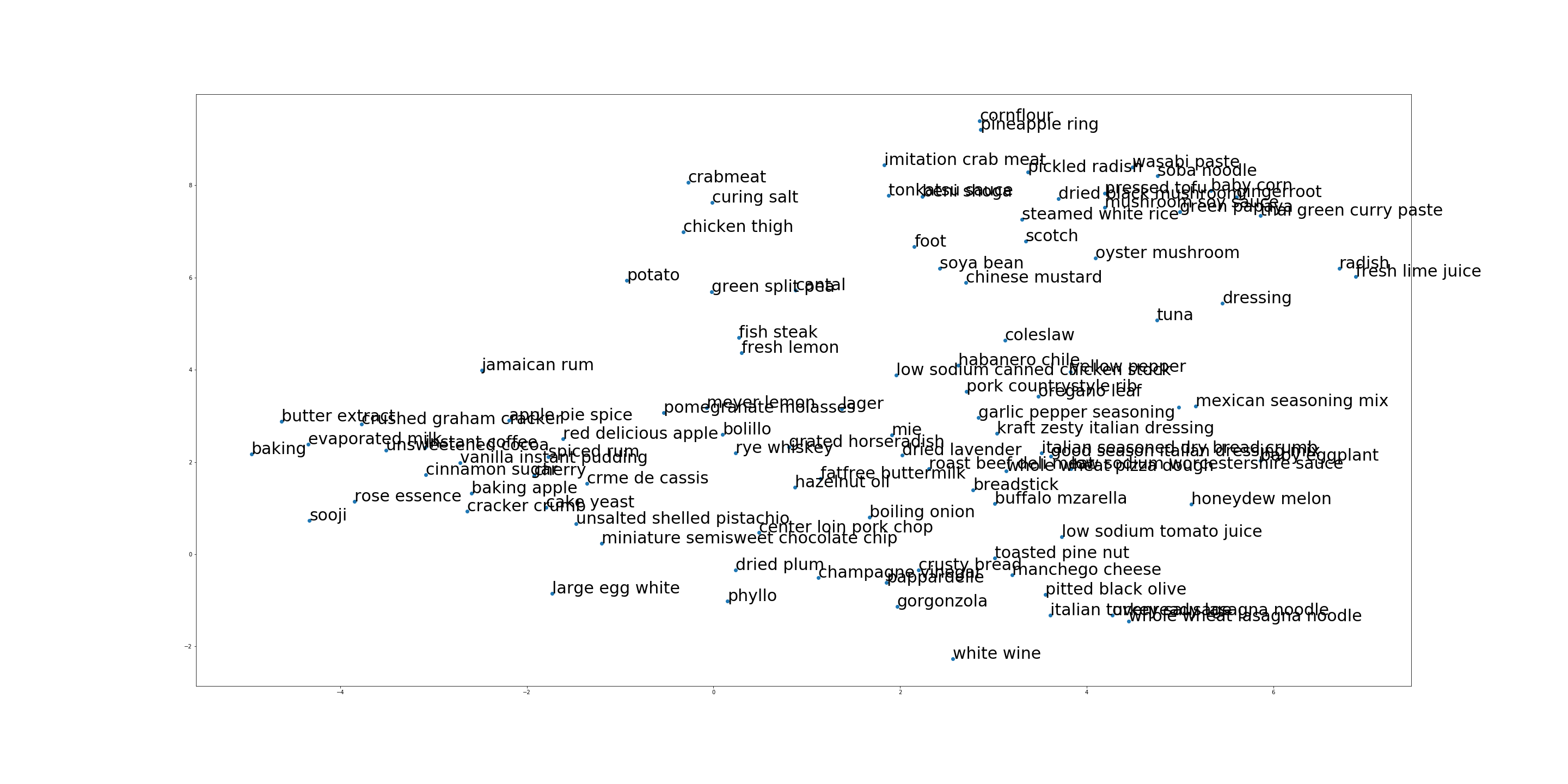
이번 포스팅에선 kaggle data를 간단하게 전처리 과정을 거쳐 gensim 의 word2vec을 이용하여 embedding vector를 만드는 과정에 대해 작성하였습니다.
다음 포스팅에선 facebook의 fasttext를 다뤄보도록 하겠습니다.